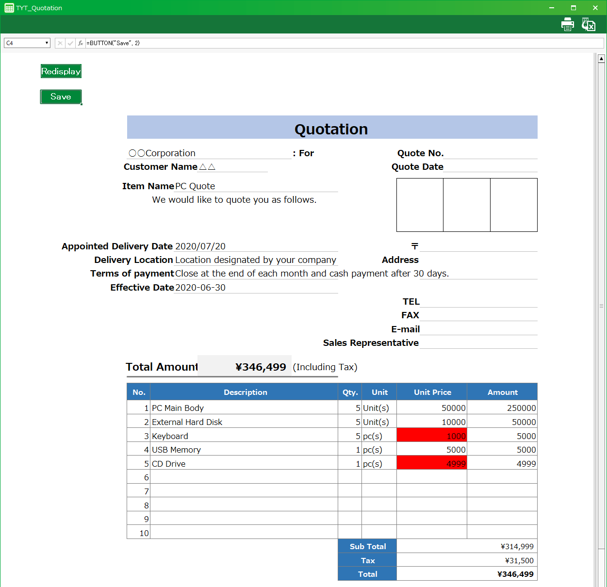
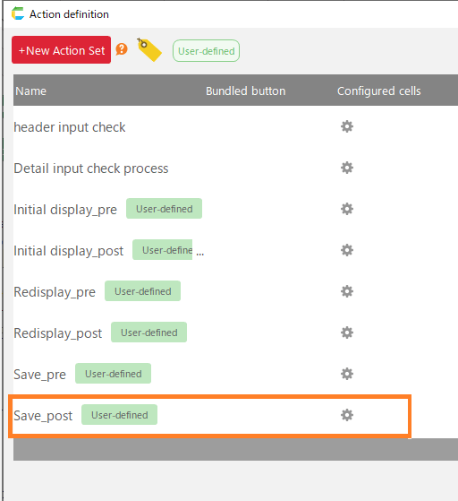
Add alert display function to single-cut screen

Data that needs to be processed urgently can be displayed in red on the single-cut screen.

Here, as an example, we will add the function to display the items whose unit price of the quotation application is below the threshold value in red.

App Operation

Items whose unit price is below 5,000 yen are displayed in red.

Customization procedure

Change screen layout

Set the threshold to display alerts on the screen.

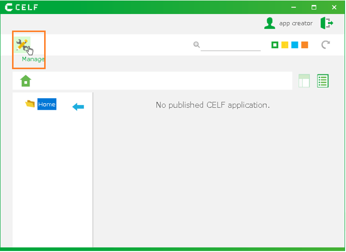
1. Login to CELF and click the "Manage"button to open the Management screen.

Tip

The "Manage" button appears when you are logged in as anadministrator.

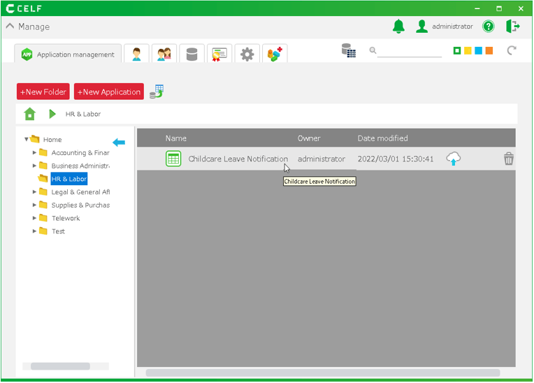
2. Double-click the app you want to customize.

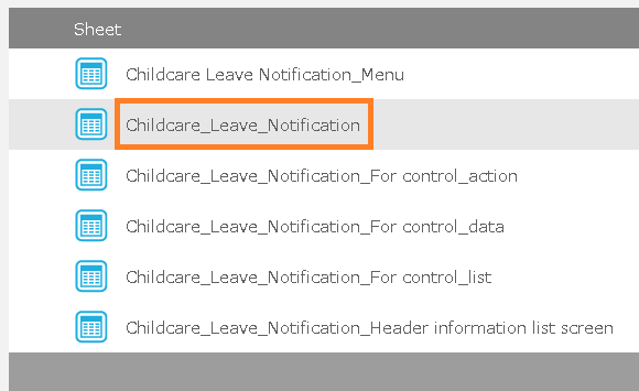
3. Double-click the quotation sheet (main sheet).

4. Click the button in the sheet setting category.

5. In the "General" tab, increase the value of "Number of columns" by 1 and click the "OK" button.

6. Enter the threshold in the first line of the rightmost column of the sheet.

Hint

Enter "5000" to "Display in red when the unit price is less than 5000 yen".

7. Right-click the column heading in the column where you entered the threshold and select "Hide".

8. Save and close the sheet.

Change the action to show rows that exceed the threshold in red

Add alert display function to "Redisplay" action of single-cut screen

The following figure shows the process flow of adding the alert feature to the "Redisplay" action.

The modifications are as follows

[1] Initialize the formatting of a cell in a table section

Add a process to initialize the formatting of cells in the table section.

This process is to avoid leaving the previous alert display on the second data search.

[2] Alert display settings

Add processing for alert display settings.

The number of rows in the table is processed to determine if the "Unit price" is below the threshold value.

If it is below the threshold, change the cell format in which the data is displayed.

Now, the steps below will show you how to actually modify the action set.

Open the action set in the single sheet screen.

1. Login to CELF and click the "Manage"button to open the Management screen.

Tip

The "Manage" button appears when you are logged in as anadministrator.

2. Double-click the app you want to customize.

3. Double-click the quotation sheet (main sheet).

4. Click the button.

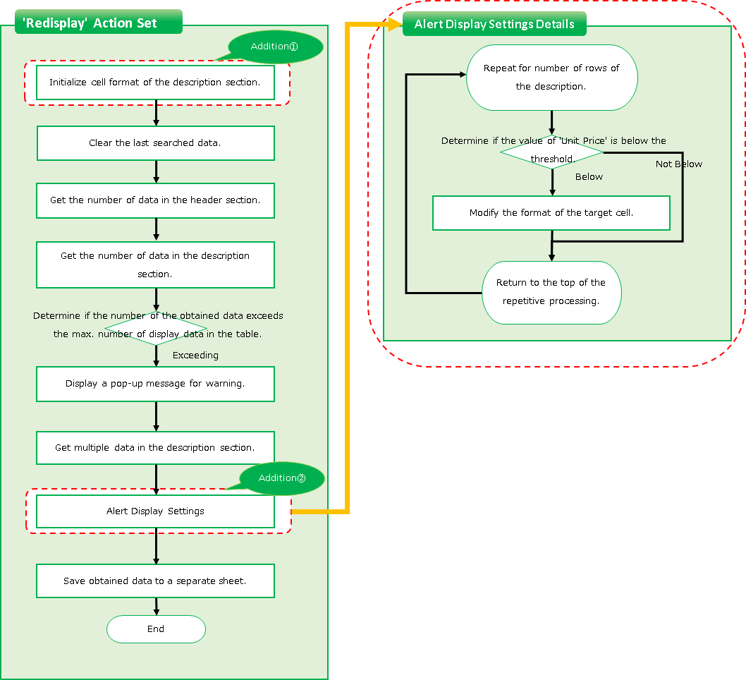
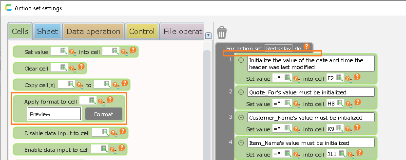
Initializing the cell formatting of a statement section

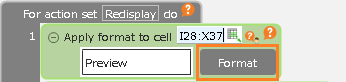
1. Double-click on the "Redisplay" action set.

2. Select the "Apply format to cell" action from the "Cells" tab and add it to the top of the action set.

Hint

The area where you can add an action will change to orange. Make sure the color of the area you want to add changes and then release the mouse button.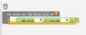

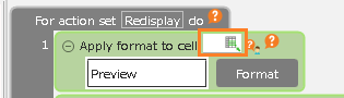
3. Click the cell selection button for the added "Apply format to cell" action.

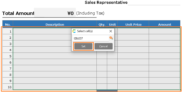
4. Select the area of the table.

5. Click the "Format" button for the added "Apply format to cell" action.

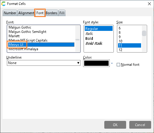
6. Edit the items in the "Font" tab as follows

• Font: MeiRyo

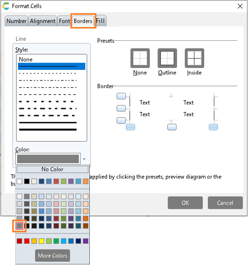
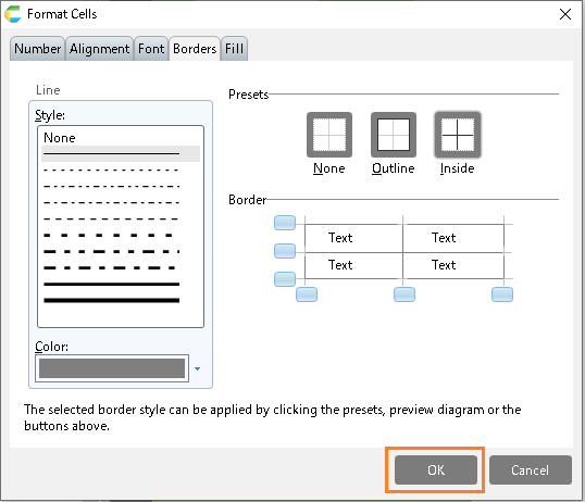
7. Edit the "Line" item on the " Borders" tab as follows.

• Color: Grey

8. Click the "Presets" item below on the " Borders" tab.

• Preset: Outline
• Preset: Inside

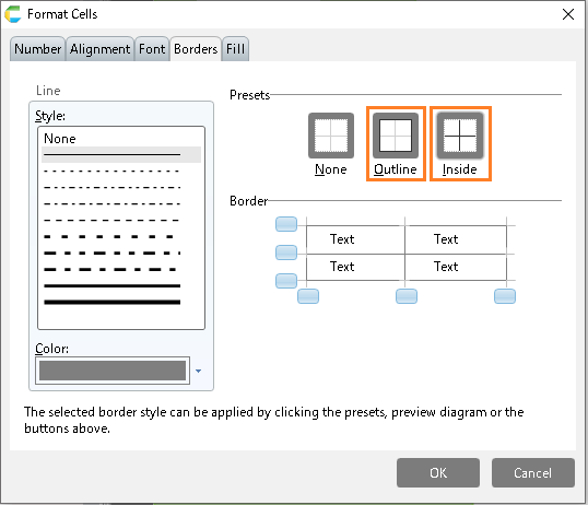
9. Click the "OK" button.

Hint

The formatting is now complete.

Add alert display function to single-cut screen

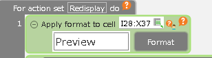
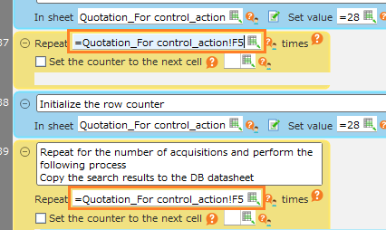
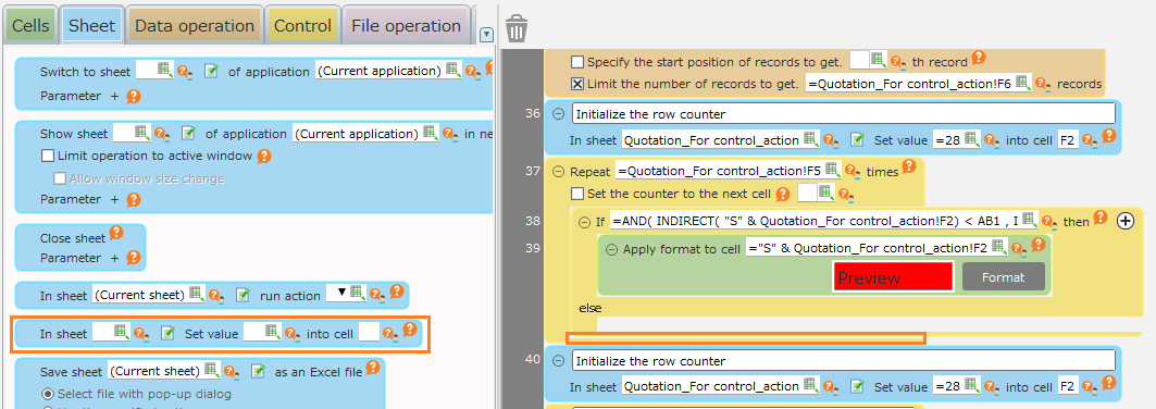
1. Copy the "Set values to sheet cell" action in line 36 by dragging and dropping it under itself.

Hint

Look for the action commented as "Initialize the row counter".

Hint

You can copy an action by dragging and dropping it while holding down Ctrl.

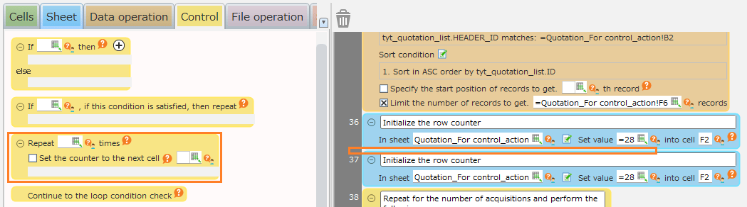
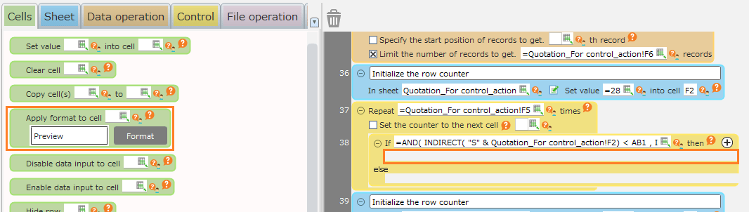
2. Add the "Repeat processing for the specified number of times" action from the "Control" tab by dragging and dropping it on top of the "Set value to sheet cell" action you copied.

3. Set the number of repetition of the added "Repeat processing for the specified number of times" action to the same formula as the number of repetitions of the "Repeat processing for the specified number of times" action 2 below.

Hint

Look for the action that is commented as follows: "Repeat for the number of acquisitions and perform the following process -Copy the search results to the DB data".

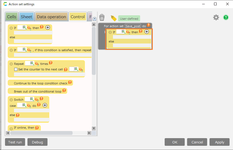
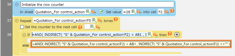
4. Select the "Determine conditions" action from the "Control" tab, and drag and drop it into the "Repeat processing for the specified number of times" action that you added.

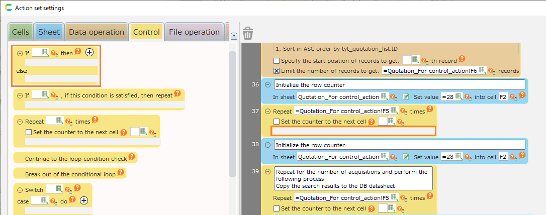
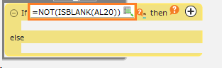
5. Enter "=AND( INDIRECT( "S" & [sheet name]!F2) < AB1 , INDIRECT( "S" & [sheet name]!F2) <>"" )" in the branching condition of the added "Determine condition" action.

Hint

This formula is complex, so please copy and paste it from the description above and make appropriate changes.

If you are interested, the meaning of the formula is explained in the "Side note".

Tip

This formula expresses the condition of a cell that is displayed with a red background color, "If the 'Unit price of that row' is below the 'Threshold' and if the 'Unit price of that row' is not blank".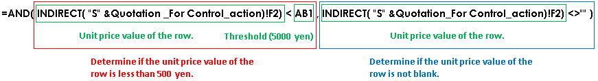

'"S" & [sheet name]!F2' represents the cell address of "Unit price of that row".

""S"" is the column address for the unit price,

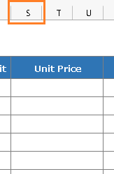and the "[sheet name]!F2" is the address of the row.

"AB1" is the address of the threshold cell set in "Change screen layout".

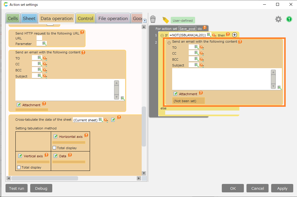
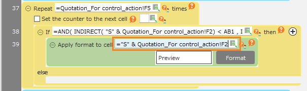
6. Select the "Apply format to cell" action from the "Cells" tab and drag and drop it onto the "If ___ then" part of the "Determine condition" action you added.

7. Enter "="S" & [sheet name]!F2" in the cell entry field of the added action.

Hint

This formula is complex, so please copy and paste it from the description above and make appropriate changes.

If you are interested, the meaning of the formula is explained in the "Side note".

Tip

'"S" & [sheet name]!F2' represents the cell address of "Unit price of that row".

""S"" is the column address for the unit price,

and the "[sheet name]!F2" is the address of the row.

8. Click the "Format" button for the added "Apply format to cell" action.

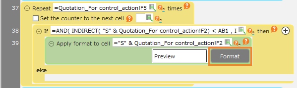
9. Edit the items in the "Font" tab as follows

• Font: MeiRyo

10. Edit the "Line" item on the " Borders" tab as follows.

• Color: Grey

11. Click the "Presets" item below on the " Borders" tab.

• Preset: Outline
• Preset: Inside

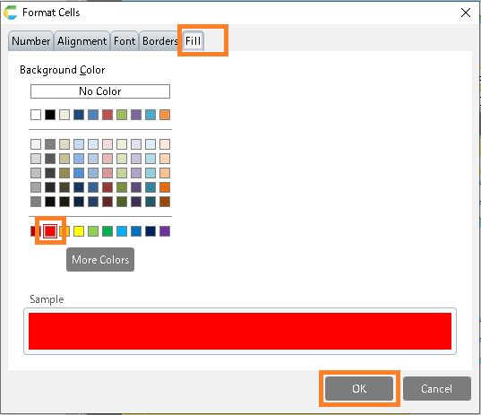
12. In the "Fill" tab, edit the "Cell Shading Color" item and click the "OK" button.

• Shaded color of the cells: red

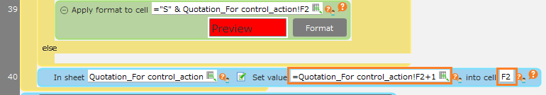
13. Select the "Set value to sheet cell" action from the "Sheets" tab and copy it by dragging and dropping it underneath the "Repeat processing for the specified number of times" action you added in step 2.

Hint

Pay close attention to the position when adding, so that it looks like the following image.

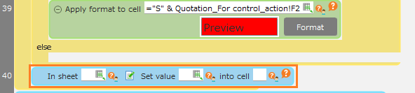
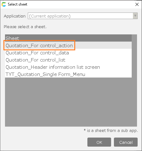
14. Click the "Select sheet"button of the added "Set value to sheet cell" action.

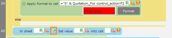
15. Double-click on the "Quotation_for Control（Action）" sheet.

16. Configure the added "Set value to sheet cell" actions as follows

• Cell: "F2"
• Value: "[sheet name]!F2 + 1"

Tip

For "[sheet name]!F2 + 1", add 1 to the row number.

This action causes the value to increase each time it is repeated with the "Repeat processing for the specified number of times" action, covering all rows in the unit price column.

17. Click the "OK" button on the action set.

Completed.

See also

Similar functionality can be added to other sheets.

To add it to the header search screen sheet, see "Add an alert display function on the header search screen".

To add to the list sheet, see "Add alert display function to list screen".

To add to a cross sheet, see "Add an alert function to the cross table screen".