Add alert display function to list screen

Data that needs to be processed urgently can be displayed in red on the list screen.

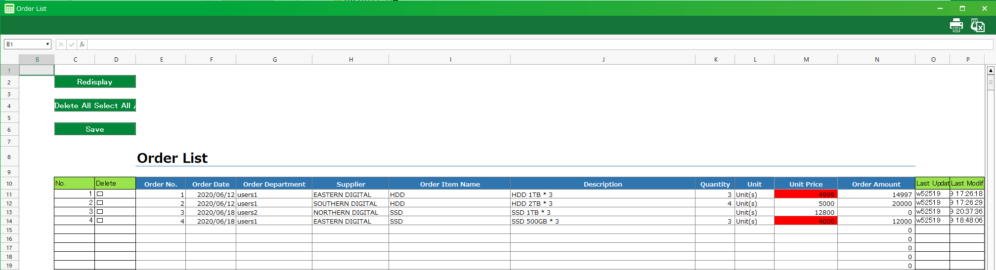
Here, as an example, we will add the function to display the items whose unit price of the order list application is below the threshold value in red.

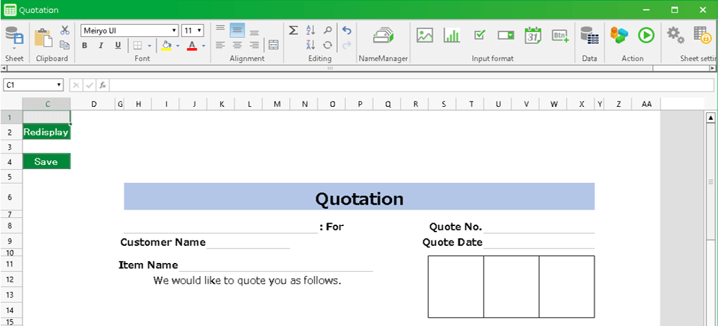
App Operation

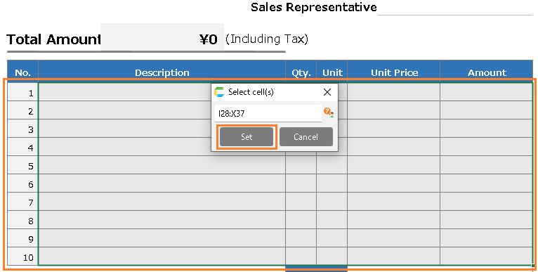
Items whose unit price is below 5,000 yen are displayed in red.

Customization procedure

Change screen layout

Set the threshold to display alerts on the screen.

1. Login to CELF and click the "Manage"button to open the Management screen.

Tip

The "Manage" button appears when you are logged in as an administrator.

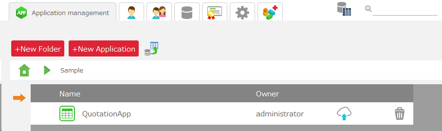
2. Double-click the app you want to customize.

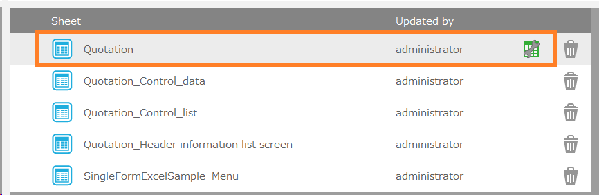
3. Double-click the Order List sheet (main sheet).

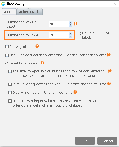
4. Click on the column heading of the last column displayed and drag it to the right.

Hint

Drag the mouse to the right of the last column.

5. With the entire last column selected, right-click on the column heading of the column and click "Unhide".

Tip

The hidden columns will be displayed.

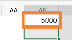
6. Enter the threshold in the first line of the displayed column.

Hint

Enter "5000" to "Display in red when the unit price is less than 5000 yen".

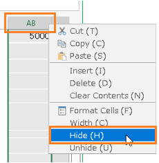
7. Right-click the column heading in the column where you entered the threshold and select "Hide".

8. Save and close the sheet.

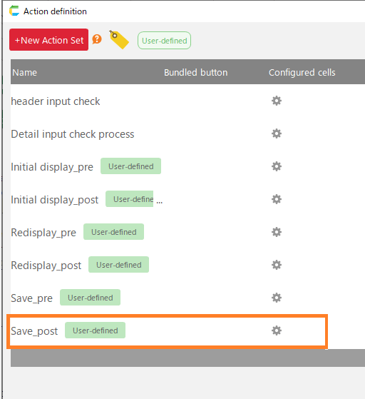
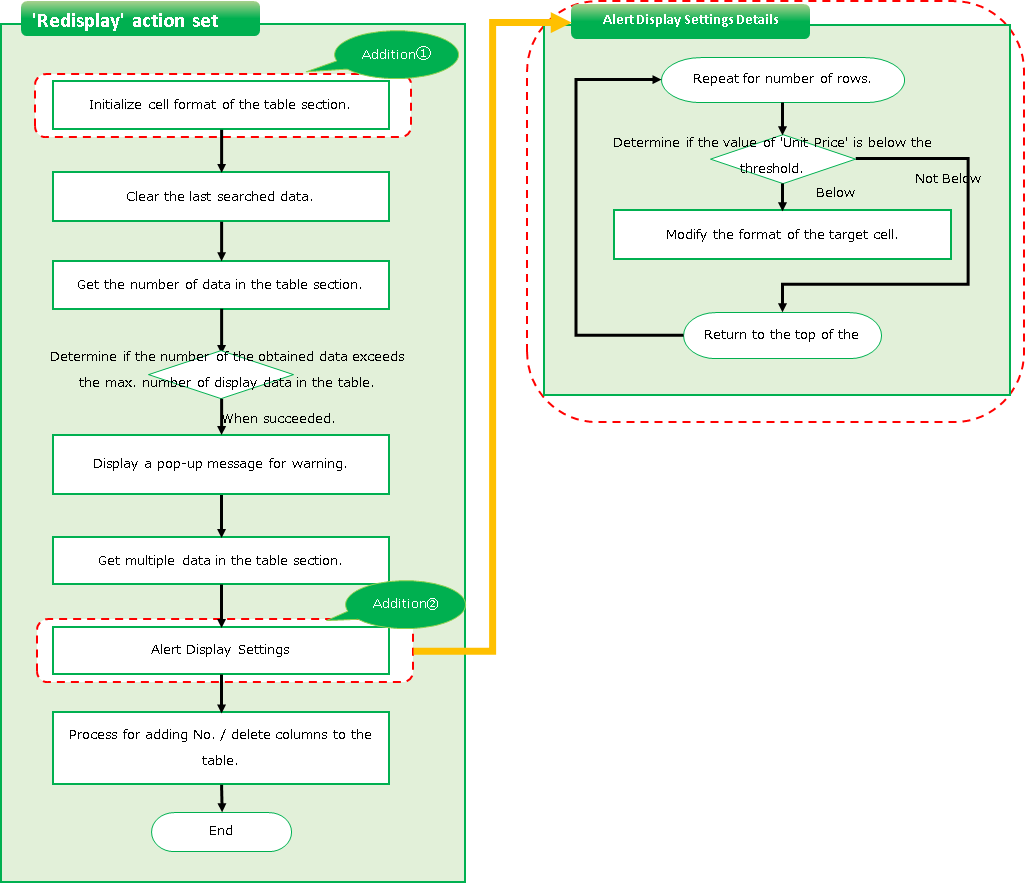
Change the action to show rows that exceed the threshold in red

Add alert display function to the "Redisplay" action of the list screen

The following figure shows the process flow of adding the alert display function to the "Redisplay" action.

The modifications are as follows

[1] Initialize the formatting of a cell in a table section

Add a process to initialize the formatting of cells in the table section.

This process is to avoid leaving the previous alert display on the second data search.

[2] Alert display settings

Add processing for alert display settings.

The number of rows in the table is processed to determine if the "Unit price" is below the threshold value.

If it is below the threshold, change the cell format in which the data is displayed.

Now, the steps below will show you how to actually modify the action set.

Open the "Redisplay" action on the list screen

1. Login to CELF and click the "Manage"button to open the Management screen.

Tip

The "Manage" button appears when you are logged in as an administrator.

2. Double-click the app you want to customize.

3. Double-click the Order List sheet (main sheet).

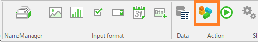
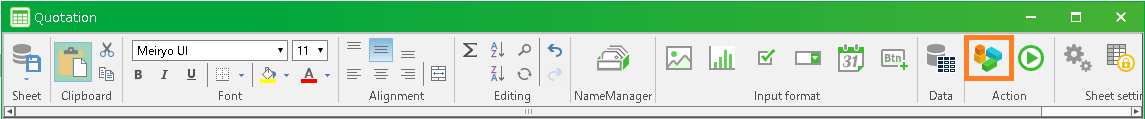
4. Click the button.

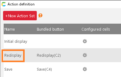
5. Double-click the "Redisplay" action set.

Initialize the cell format of a table section

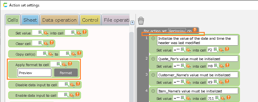
1. Select the "Set cell format" action from the "Cells" tab and add it by dragging and dropping it to the top of the action set.

Hint

The area where you can add an action will change to orange. Make sure the color of the area you want to add changes and then release the mouse button.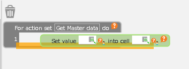

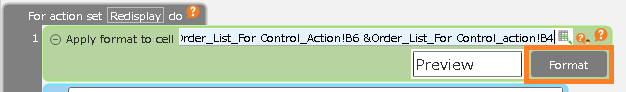
2. In the added "Set cell format" action, enter '=[sheet name]!B5 & [sheet name]!B3 & "":" & [sheet name]!B6 & [sheet name]!B4'.

Hint

This formula is complex, so please copy and paste it from the description above.

The meaning of the formula is explained in the "Side note" section below, if you’re interested.

Tip

This formula represents the range of the list, "From "Cell address at the start of the table" to "Cell address at the end of the table"".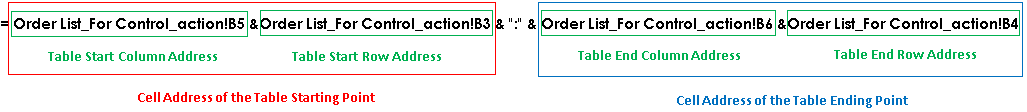

The "Cell address at the start of the table" indicates the following cells

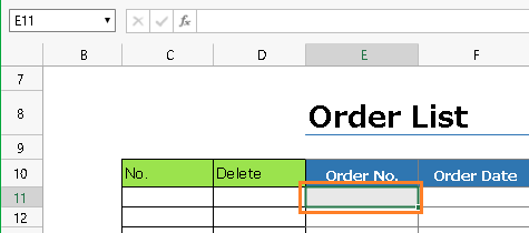The "Cell address at the end of the table" indicates the following cells

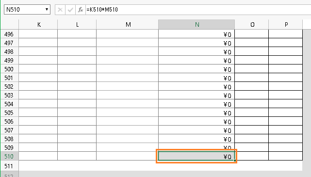
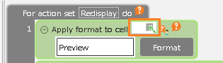
3. Click the "Format" button for the added "Set cell format" action.

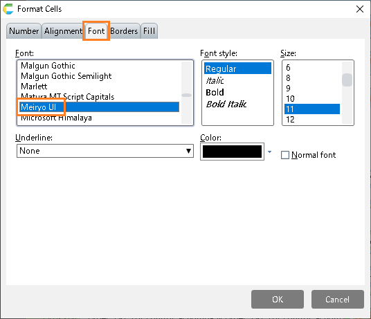
4. Edit the items in the "Font" tab as follows

• Font: MeiRyo

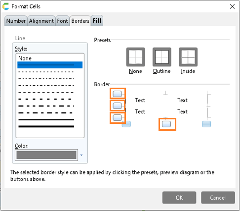
5. Use the "Borders" tab to set the left and right borders.

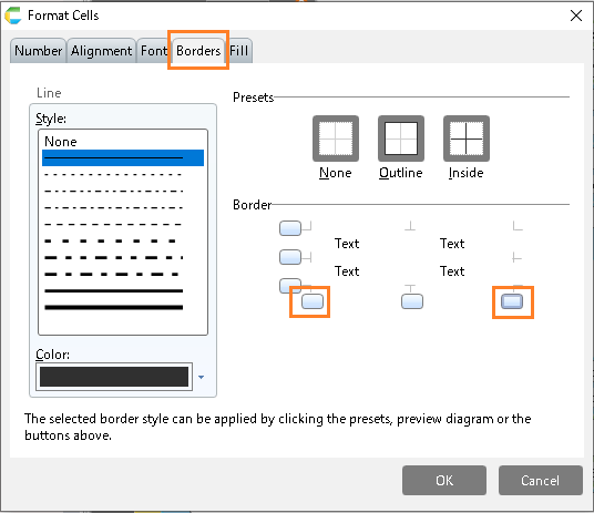
Hint

Black lines will appear on the left and right.

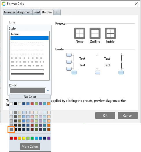
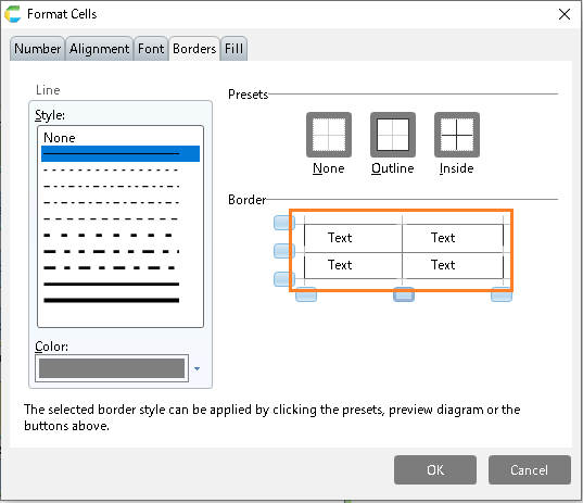
6. On the "Borders" tab, set the color of the line to gray.

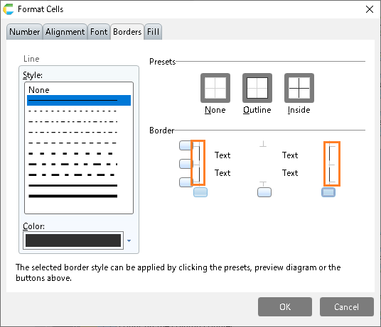
7. On the "Borders" tab, set the remaining borders in step 10.

Hint

A gray line will appear.

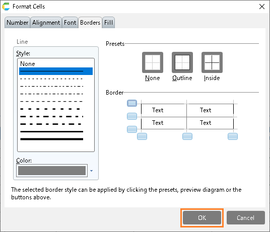
8. Click the "OK" button.

Add alert display function to list screen

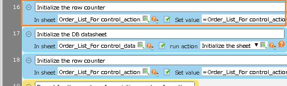
1. Copy the "Set value to sheet cell" action on line 17 by dragging and dropping it on top of the previous "Execute sheet action" action.

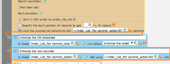
Hint

Make sure you copy it into the following image, taking care to position it so that it looks like the following image.

Hint

You can copy an action by dragging and dropping it while holding down Ctrl.

2. Add the "Repeat processing for the specified number of times" action from the "Control" tab by dragging and dropping it under the "Set value to sheet cell" action that you copied.

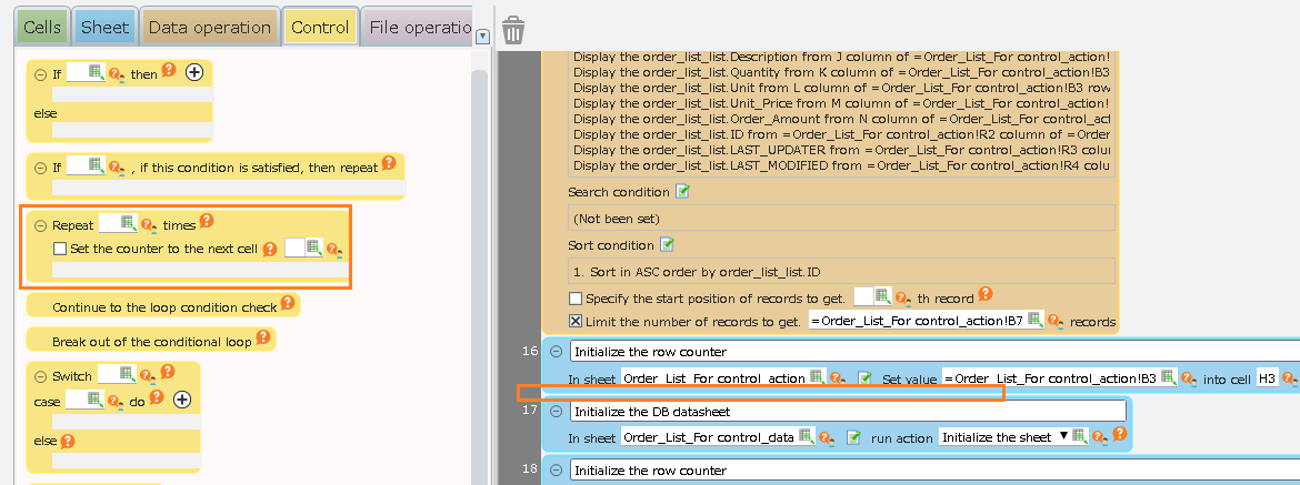
3. Set the number of repetition of the added "Repeat processing for the specified number of times" action to the same formula as the number of repetitions of the "Repeat processing for the specified number of times" action 3 below.

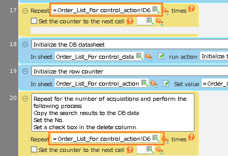
Hint

Look for the actions listed in the comments below.

Repeat for the number of acquisitions and perform the following process

・Copy the search results to DB data

・Set No.

・Set the checkboxes in the Delete column.

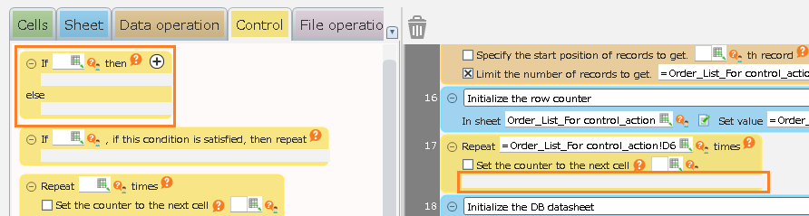
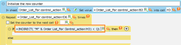
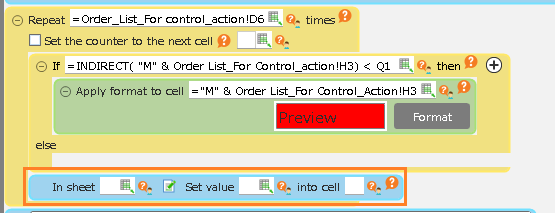
4. Drag and drop the "Determine condition" action from the "Control" tab into the "Repeat processing for the specified number of times" action that you added.

5. Enter "=INDIRECT( "M" & [sheet name]!H3) < Q1" in the branching condition of the added "Determine condition" action.

Hint

This formula is complex, so please copy and paste it from the description above.

The meaning of the formula is explained in the "Side note" section below, if you’re interested.

Tip

This formula expresses the condition of a cell that is displayed with a red background color, "If the 'Unit price of that row' is below the 'Threshold'".

""M" & [sheet name]!H3" represents the cell address of "Unit price of that row".

The ""M"" is the unit price column address,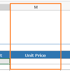

The "[sheet name]!H3" displays the address of the row.

"Q1" is the address of the threshold cell set by Change screen layout.

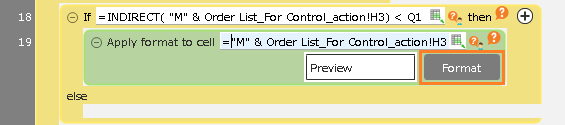
6. Select the "Set cell format" action from the "Cells" tab and drag and drop it onto the "If ___ then" part of the "Determine condition" action you added.

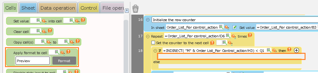
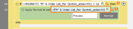
7. Enter "="M" & [sheet name]!H3" in the cell input field of the added "Set cell format" action.

Hint

If you are interested, the meaning of the formula is explained in the "Side note" section of Procedure 5.

8. Click the "Format" button for the added "Set cell format" action.

9. Edit the items in the "Font" tab as follows

• Font: MeiRyo

10. Edit the "Lines" item on the "Borders" tab as follows.

• Color: Grey

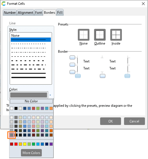
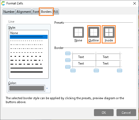
11. Click the "Presets" item below on the "Borders" tab.

• Preset: Outline
• Preset: Inside

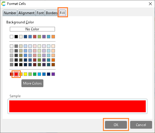
12. In the "Fill" tab, edit the "Cell Shading Color" item and click the "OK" button.

• Shaded color of the cells: red

13. Select the "Set value to sheet cell" action from the "Sheets" tab and copy it by dragging and dropping it underneath the "Repeat processing for the specified number of times" action you added in step 2.

Hint

Pay close attention to the position when adding, so that it looks like the following image.

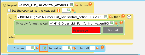
14. Click the "Select sheet" button of the added "Set value to sheet cell" action.

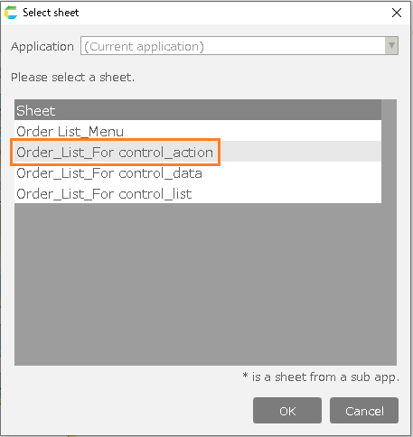
15. Double-click the "Order List__for Control(Action)" sheet.

16. Configure the added "Set value to sheet cell" actions as follows.

• Cell: "H3"
• Value："=[sheet name]!H3 + 1"

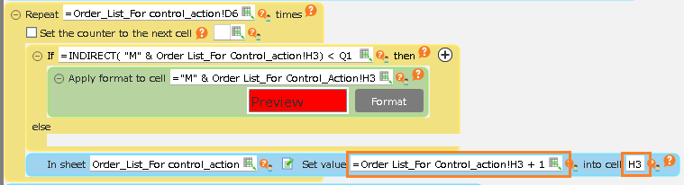
Tip

For "=[sheet name]!H3 + 1", add 1 to the row number.

This action causes the value to increase each time it is repeated with the "Repeat processing for the specified number of times" action, covering all rows in the unit price column.

17. Click the "OK" button on the action set.

Completed.

See also

Similar functionality can be added to other sheets.

To add it to the header search screen sheet, see "Add an alert display function on the header search screen".

To add to a single sheet, see "Add alert display function to single-cut screen".

To add to a cross sheet, see "Add an alert function to the cross table screen".