Add an alert display function on the header search screen

Data that needs to be processed urgently can be displayed in red on the header search screen.

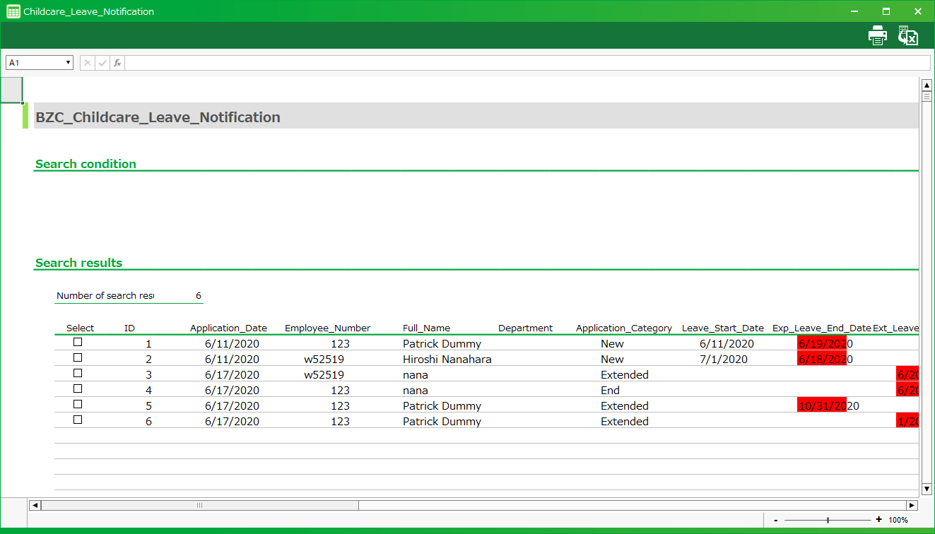
As an example, in the header list of the Parental Leave Application, we will add a function to display the applications in red, whose scheduled end date of leave is earlier than today’s date.

App Operation

The "Scheduled end date of leave" in the row of the leave notification that the end date of leave has passed is displayed in red.

Customization procedure

Change screen layout

Set the threshold to display alerts on the screen.

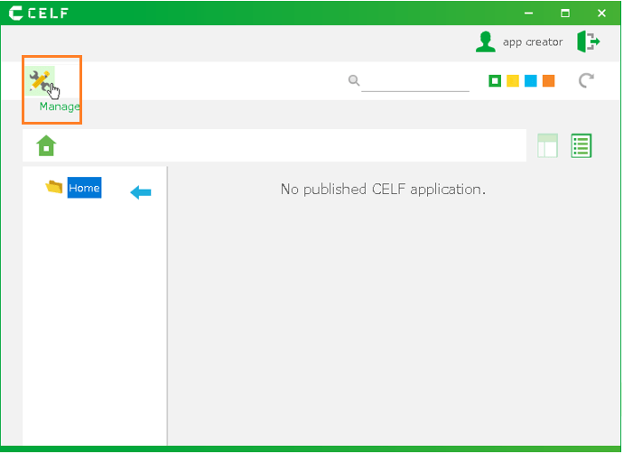
1. Login to CELF and click the "Manage"button to open the Management screen.

   

   Tip

   The "Manage" appears when you are logged in as an administrator.

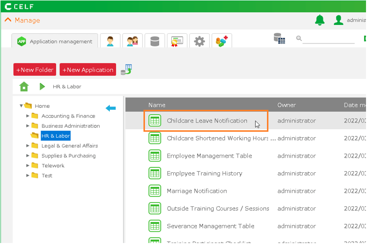
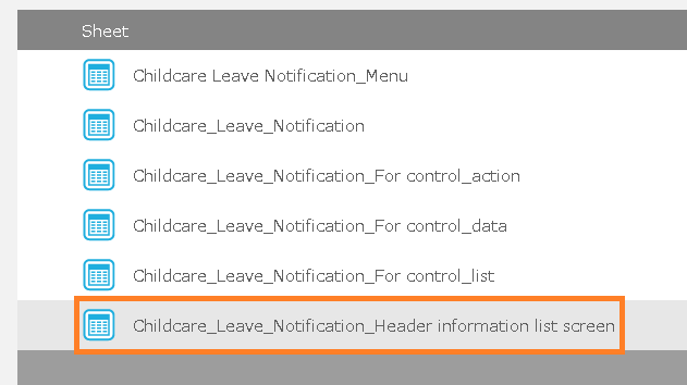
2. Double-click the app you want to customize.

   

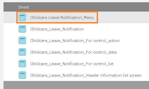
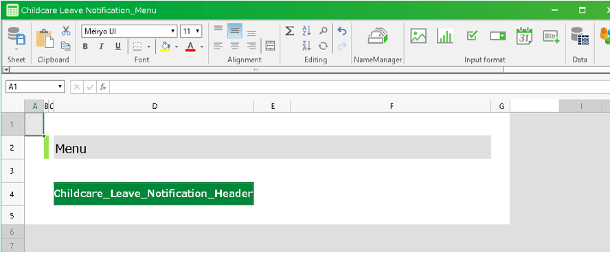
3. Double-click the menu sheet.

   

   Hint

   A sheet with the name "[app name]_menu" is a menu sheet.

   Tip

   Here we set the thresholds on the menu screen to reference from all sheets.

   You can also set the threshold in the header search screen in the same way.

4. Click the button.

   

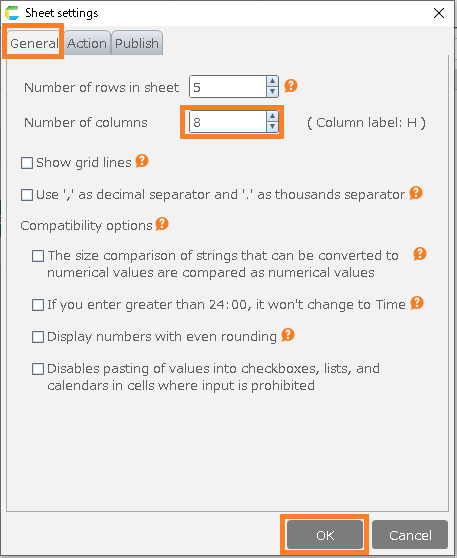
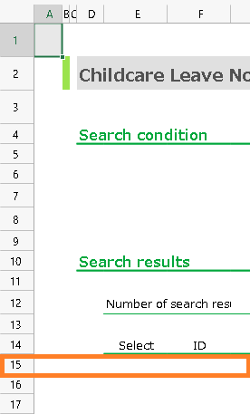
5. In the "General" tab, increase the value of "Number of columns" by 1 and click the "OK" button.

   

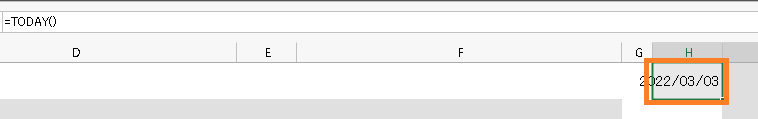
6. Enter "=TODAY()" in the first cell of the first row of the added column.

   

   Hint

   All expressions must be entered in half-width characters.

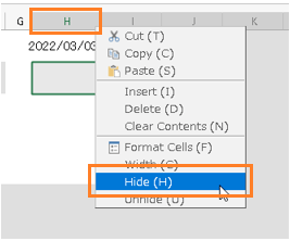
7. Right-click on the column heading of the column in which you entered the expression and select "Hide".

   

8. Save and close the sheet.

   

Change the action to show rows that exceed the threshold in red

Add an alert display function to the "List view" action from the header search screen.

The following figure shows the process flow of adding the alert feature to the "List view" action.

The modifications are as follows

[1] Alert display settings

Add processing for alert display settings.

Process the number of acquired data and determine whether the value of the "Scheduled end date of leave" is below the threshold.

If it is below the threshold, change the cell format in which the data is displayed.

Now, the steps below will show you how to actually modify the action set.

Open the action set in the header search screen.

1. Double-click the header search screen sheet.

   

   Hint

   The sheet named "[App Name]_Header Screen" is the Header Search Screen Sheet.

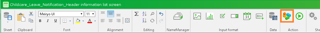
2. Click the button.

   

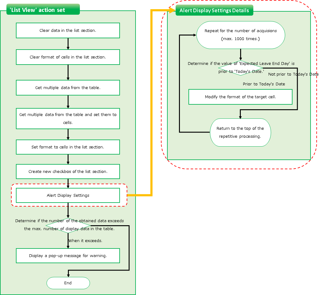
Add an alert on the header search screen

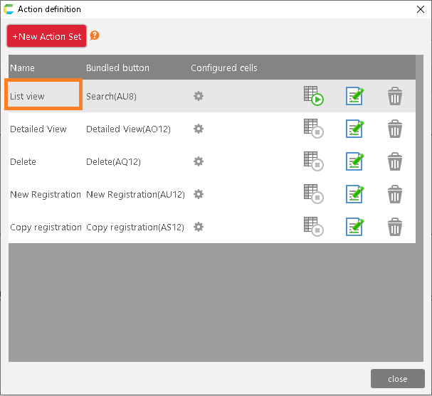
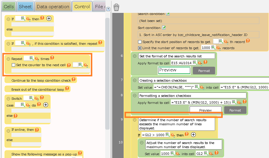
1. Double-click on the "List view" action set.

   

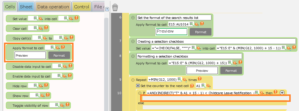
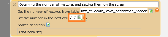
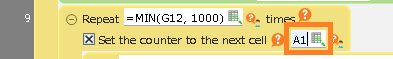
2. Add the "Repeat processing for the specified number of times" action between lines 8 and 9.

   

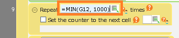
3. Enter "=MIN(G12, 1000)" in the repeat count.

   

   Tip

   In this expression, the address (G12) uses the address that is set to the number of cases retrieved from the table in "Get number of records from table" in line 3.

   

   Hint

   All expressions must be entered in half-width characters.

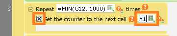
4. Check the "Set the counter to the next cell" checkbox and enter "A1" in the address box.

   

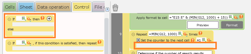
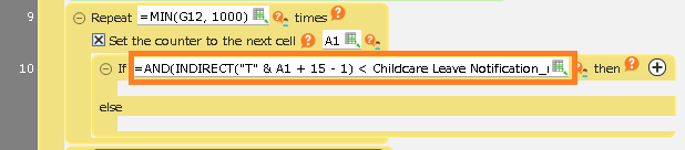
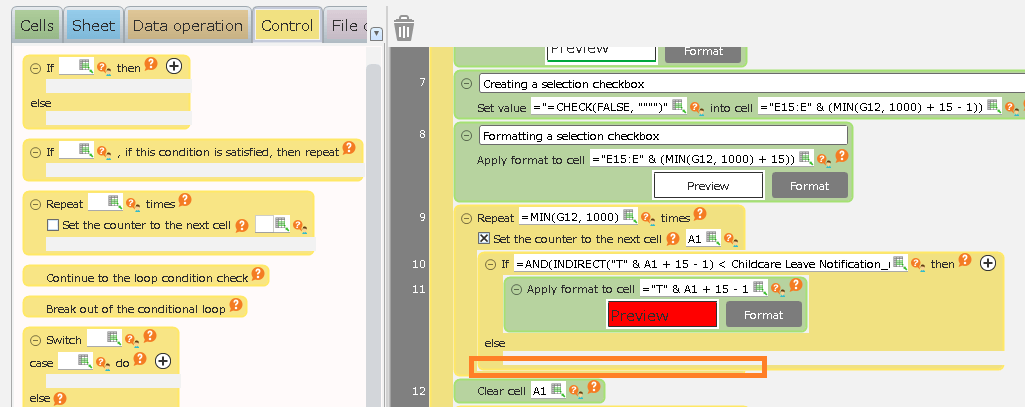
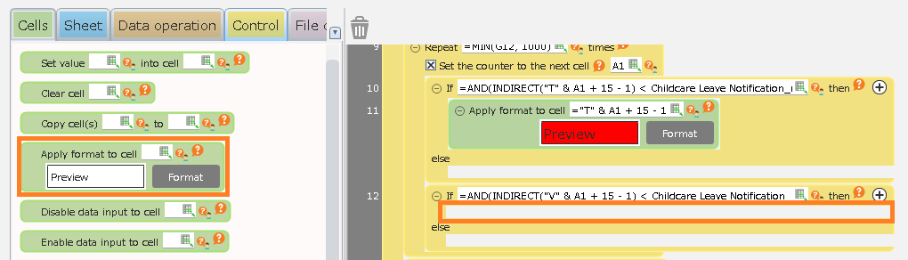
5. Set the "Determine condition" action in the "Repeat processing for the specified number of times" action in row 9.

   

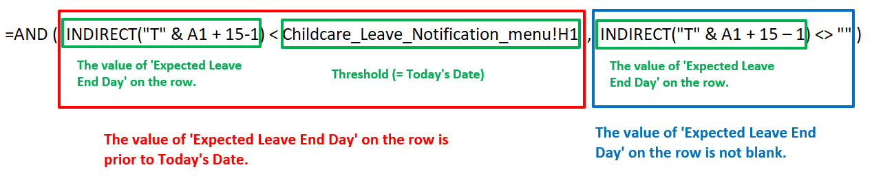
6. Enter the expression "=AND(INDIRECT("T" & A1 + 15 - 1) <[sheet name]!H1, INDIRECT("T" & A1 + 15 - 1) <> "")" in the condition of the "Determine condition" action you added.

   

   Hint

   This formula is complex, so please copy and paste it from the description above.

   The meaning of the formula is explained in the "Tip"' section below, if you’re interested.

   Tip

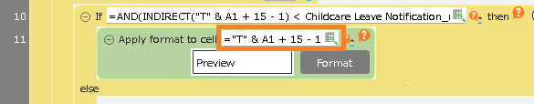
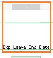
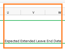
   This formula represents the condition 'If the "End date of parental leave in that row" is less than the "Threshold" and the "End date of parental leave in that row" is not blank', the cell is displayed with a red background.

   

   
   

   '"T" & A1 + 15 - 1' represents the cell address of the"End date of parental leave in that row.

   "T" is the column address for the end date of parental leave,

   

   "15" is the row number of the first row of the search results list,

   

   "A1" is the number of cases on the list that we are currently determining.

   

   
   

   "[sheet name]!H1" is the address of the threshold cell that was set in the screen layout change earlier.

7. Set the "Apply format to cell" action in the first section of "Determine condition" action you just added.

   

8. Enter "="T" & A1 + 15 - 1" in the address of the cell where the format should be set.

   

   Tip

   '"T" & A1 + 15 - 1' represents the cell address of the"End date of parental leave in that row.

   "T" is the column address for the end date of parental leave,

   

   "15" is the row number of the first row of the search results list,

   

   "A1" is the number of cases on the list that we are currently determining.

   

9. Click the "Format" button.

   

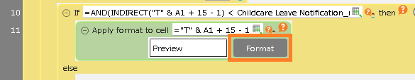
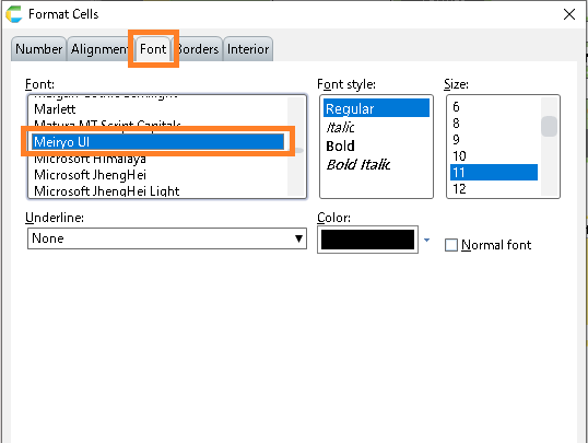
10. In the "Fonts" tab, select "MeiRyo" for "Fonts".

    

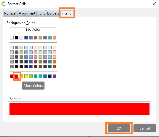
11. In the "Fill" tab, select red for the "Shading Color for Cells" and click the "Confirm" button.

    

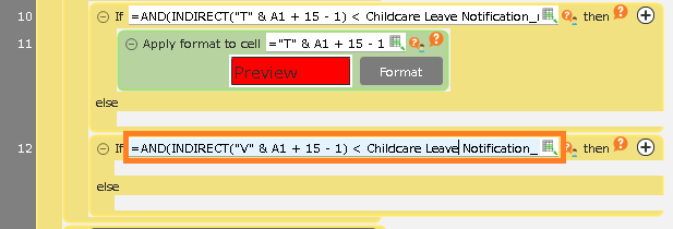
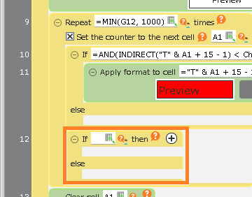
12. Set the "Determine condition" action in the "Repeat processing for the specified number of times" action in row 9.

    

    Hint

    Pay close attention to the position when adding, so that it looks like the following image.

    

13. Enter "=AND(INDIRECT("V" & A1 + 15 - 1) < Parental Leave Application_Menu!H1, INDIRECT("V" & A1 + 15 - 1) <> "")" as a condition for the added "Determine condition" action.

    

    Hint

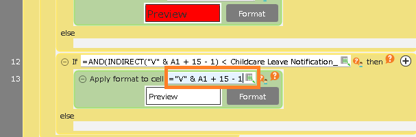
    This formula is complex, so please copy and paste it from the description above.

    The meaning of the expression is the same as in Section 8. Only the column address is changed from "T" to "V" because the item that changes the background color isdifferent.

    

    If you are interested, please see "Tip" for details on the meaning of the expression.

14. Set the "Apply format to cell" action in the first section of "Determine condition" action you just added.

    

15. Enter "="V" & A1 + 15 - 1" in the address of the cell where the format should be set.

    

    Tip

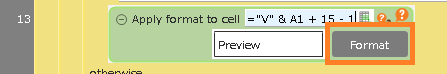
    The meaning of the expression is the same as 10.

    Because of the different settings, the address is changed from "T" to "V".

    

16. Click the "Format" button.

    

17. In the "Fonts" tab, select "MeiRyo" for "Fonts".

    

18. In the "Fill" tab, select red for the "Shading Color for Cells" and click the "Confirm" button.

    

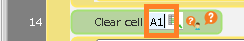
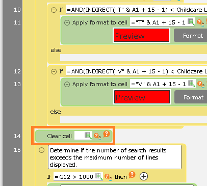
19. Add the action "Clear cell value" next to the action "Repeat processing for the specified number of times".

    

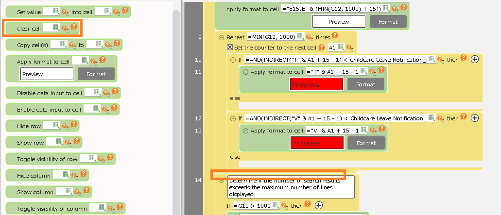
    Hint

    Pay close attention to the position when adding, so that it looks like the following image.

    

20. Enter "A1" as the cell address for the "Clear cell value" action you added.

    

21. Click the "OK" button to close the Action Set Settings dialog.

    

22. Click the "OK" button to close the Action Set Settings dialog.

    

23. Save and close the sheet.

Completed.

See also

Similar functionality can be added to other sheets.

To add to the list sheet, see "Add alert display function to list screen".

To add to a single sheet, see "Add alert display function to single-cut screen".

To add to a cross sheet, see "Add an alert function to the cross table screen".