Add an alert function to the cross table screen
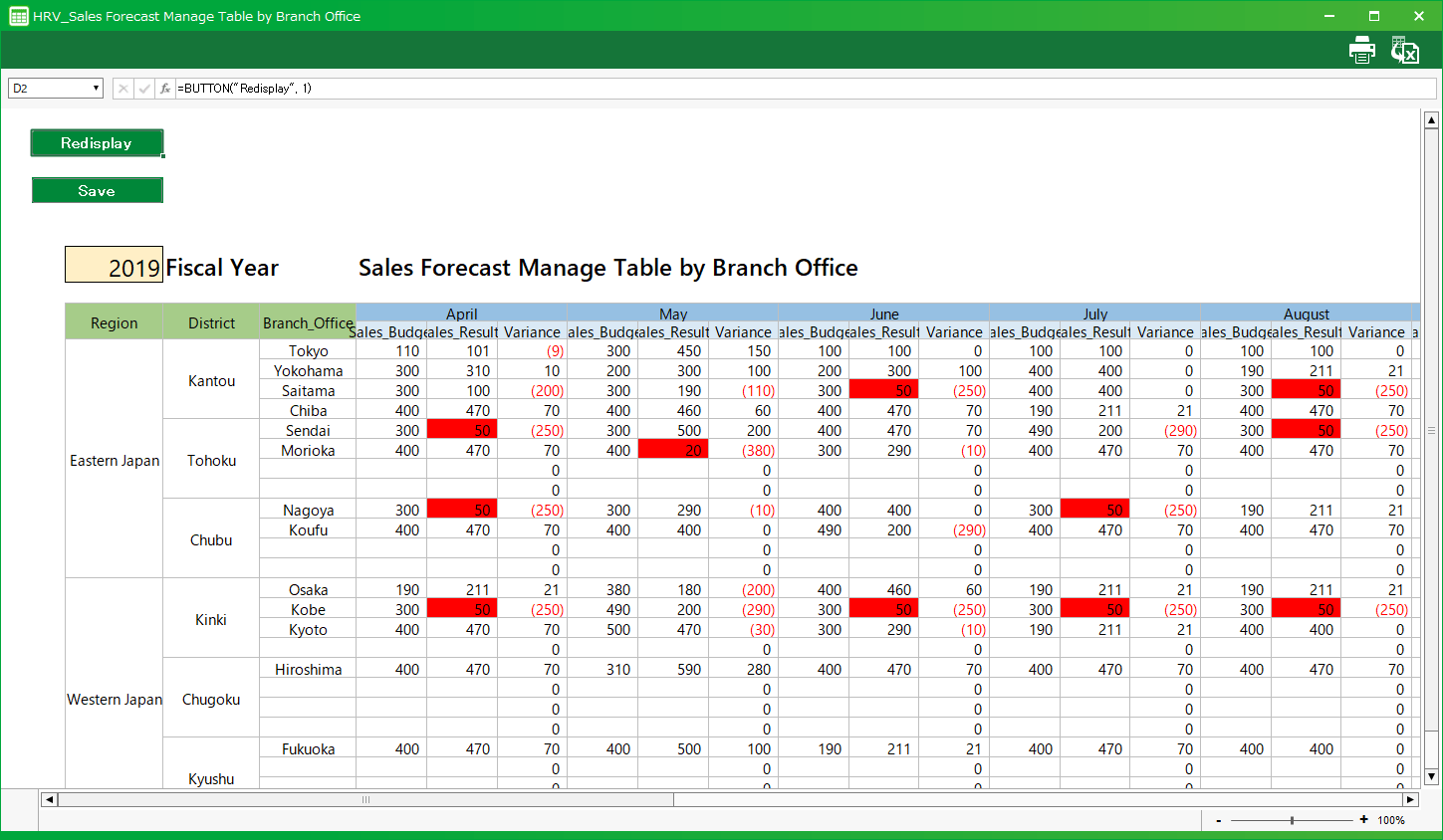
In the cross table screen, data that needs to be processed urgently can be displayed in red.
Here, as an example, a function is added to the Sales by Branch Offices sheet that displays in red when the sales result is less than 100.
Customization procedure
Change screen layout
Set the threshold to display alerts on the screen.
- Login to CELF and click the "Manage" button to open the Management screen.
Tip
The "Manage" button appears when you are logged in as anadministrator.
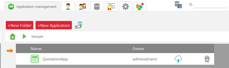
- Double-click the app you want to customize.
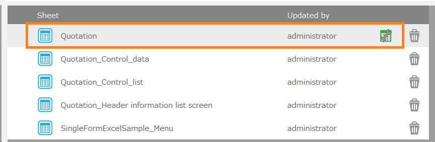
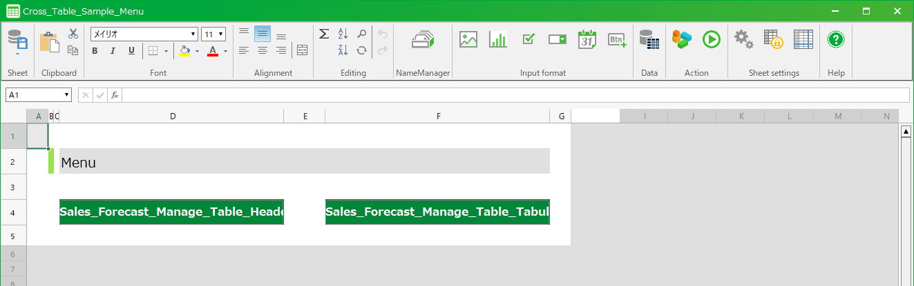
- Double-click the menu sheet.
Hint
A sheet with the name "[app name]_menu" is a menu sheet.
- Click the
 button in the sheet setting category.

- Add one sheet column.
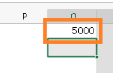
- Enter the threshold in the first line of the rightmost column of the sheet.
Hint
In this example, enter "100" to "Display in red if it is less than 100".
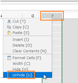
- Right-click the column heading in the column where you entered the threshold and select "Hide".
- Save and close the sheet.
Change the action to show rows that exceed the threshold in red
Open the action set on the cross table screen.
- Login to CELF and click the "Manage" button to open the Management screen.
Tip
The "Manage" button appears when you are logged in as anadministrator.
- Double-click the app you want to customize.
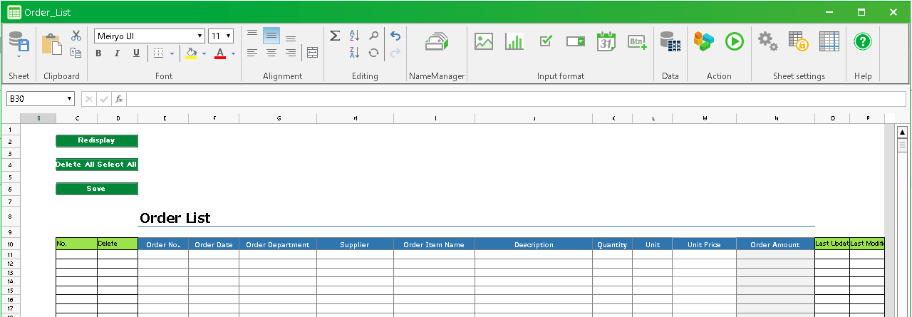
- Double-click on the main sheet.

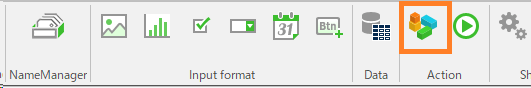
- Click the
 button.

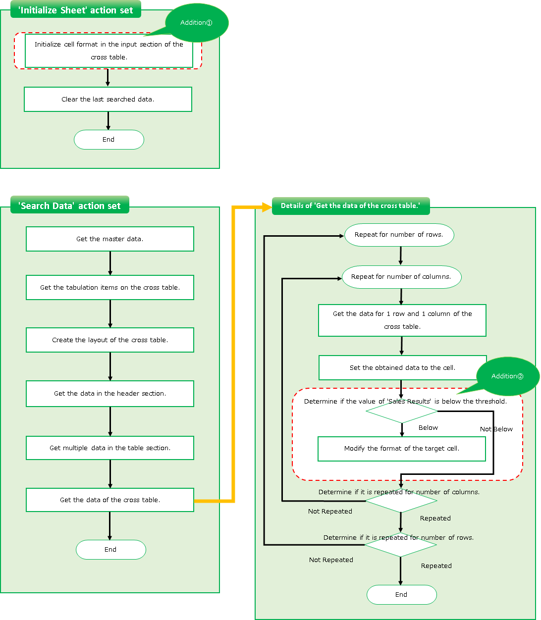
Initializing Cross Table Cell Formatting
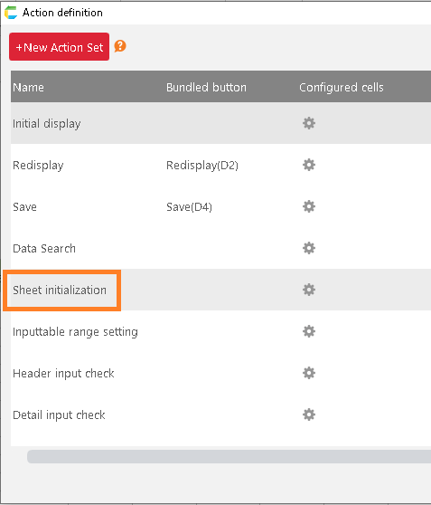
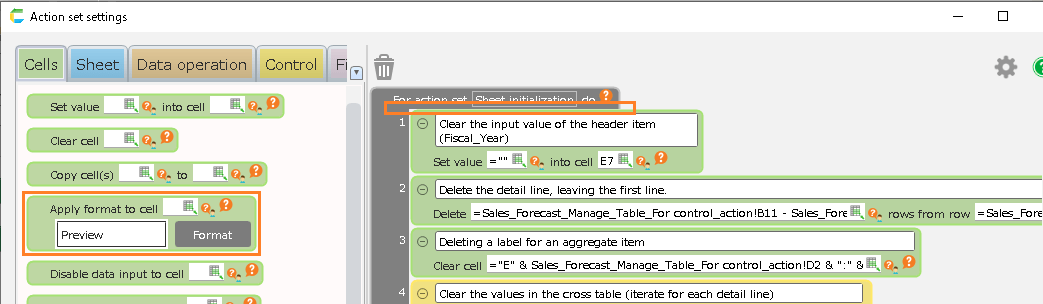
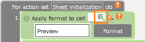
- Double-click on the "Sheet initialization" action set.
- Select the "Set cell format" action from the "Cells" tab and add it to the top of the action set.
Hint
The area where you can add an action will change to orange. Make sure the color of the area you want to add changes and then release the mouse button.
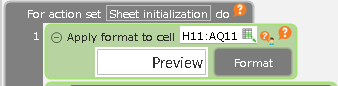
- Click the cell selection button for the added "Set cell format" action.
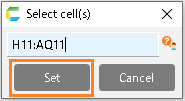
- Select the area of the table.
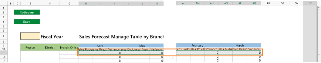
Hint
Select the first row of the table from the start to the end column of the table.
- Click the "Set" button.
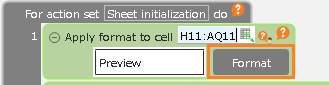
- Click the "Format" button for the added "Set cell format" action.
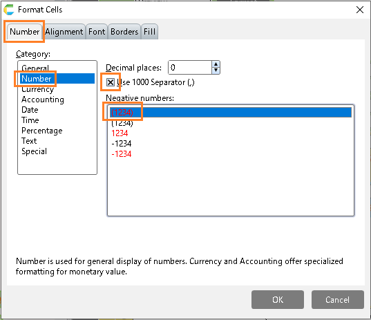
- Edit the item in the "Number" tab as follows
- Category: Number
- Use (,) for digit separator: Checked
- Negative number display format: (1234)
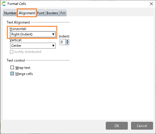
- Edit the item in the "Alignment" tab as follows
- Horizontal : Align text Right (indent)
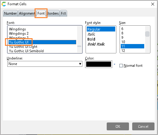
- Edit the items in the "Font" tab as follows
- Font: Yu Gothic UI
- Edit the "Lines" item on the "Borders" tab as follows.
- Color: Grey
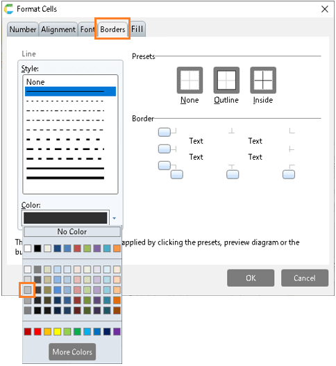
- Click the "Presets" item below on the "Borders" tab.
- Preset: Outline
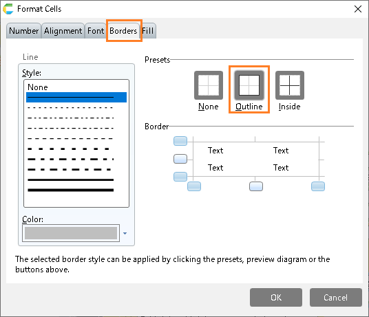
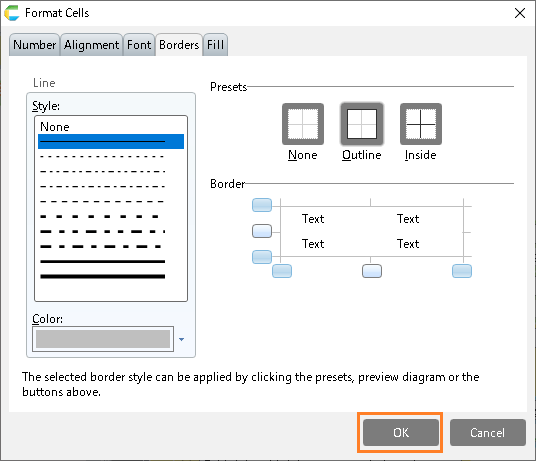
- Click the "OK" button.
Hint
The formatting is now complete.
Tip
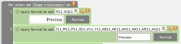
If you find non-numeric items in the area you set up in step 8, you need to add the following actions.Example: If the "Difference" item in the table is in string format
- From the "Cells" tab, add the "Set cell format" action under the action you added in step 2.
- In the cell you want to format, set the "Difference" cell for 12 months.
Hint
You can select multiple cells by selecting them while holding down the Ctrl key.
- Specify the "Categorization" item in the "Number" tab as a string.
Hint
For the other items, set up in the same way as steps 12. to 16.
- Click the "OK" button on the "Sheet initialization" action set.
Add an alert function to the cross table screen
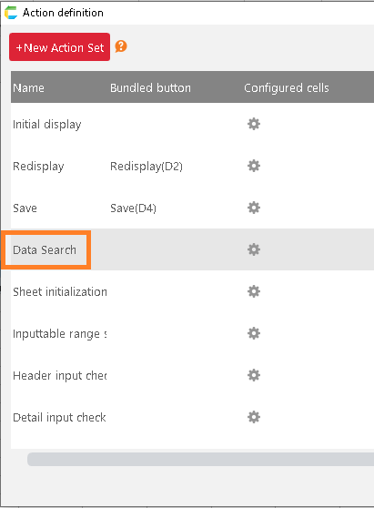
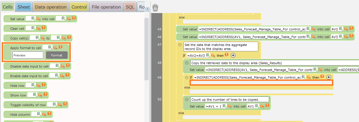
- Double-click on the "Data Search" action set.
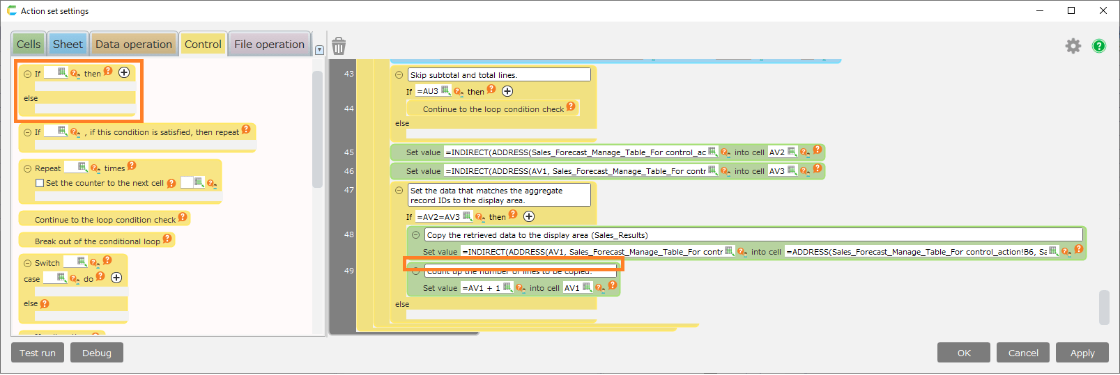
- Select the "Determine condition" action from the "Control" tab and add it by dragging and dropping it under the "Set value to cell" action.
Hint
Set the data that matches the aggregate record IDs to the display area.
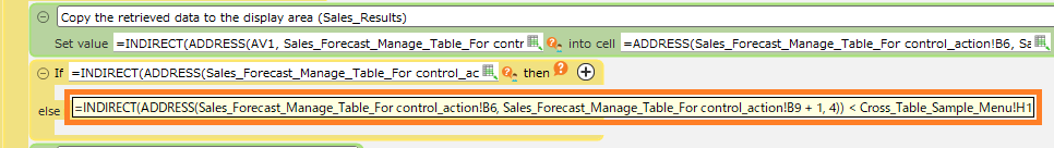
- Enter "=INDIRECT( ADDRESS([sheet name]_control(action)!B6, [sheet name]_control(action)!B9 + 1, 4) ) < [app name]_menu!H1" in the branch condition of the "Determine condition" action.
Hint
This formula is complex, so please copy and paste it from the description above and make appropriate changes.The meaning of the formula is explained in the "Side note" section below, if you’re interested.Hint
The example shows the condition of a cell with a red background: "If the sales performance of the row is less than the threshold". "[sheet name]!B6" and "[sheet name]!B9" indicatethe target row address and target column address.The "[app name]_menu!H1" is the address of the threshold cell set in Change screen layout.
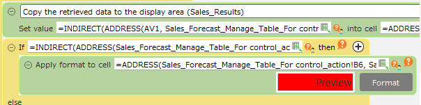
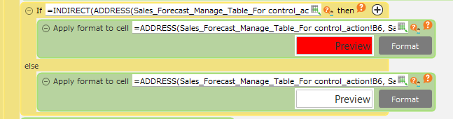
- Select the "Set cell format" action from the "Cells" tab and drag and drop it onto the "If ~ then" part of the "Determine condition" action you added.
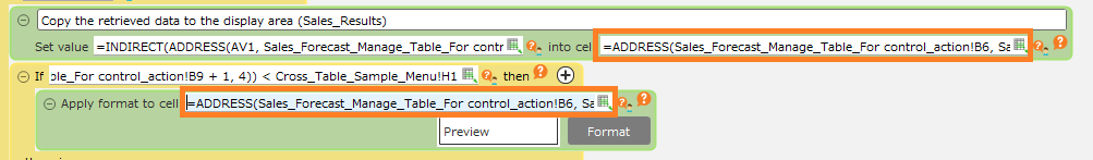
- In the cell entry field of the added action, copy the formula entered in the cell that sets the value of the previous "Set value in cell" action.
Hint
Set the data that matches the aggregate record IDs to the display area.
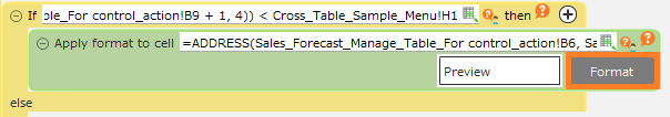
- Click the "Format" button for the added "Set cell format" action.
- Edit the item in the "Number" tab as follows
- Category: Number
- Use (,) for digit separator: Checked
- Negative number display format: (1234)
- Edit the item in the "Alignment" tab as follows
- Horizontal : Align text Right (indent)
- Edit the items in the "Font" tab as follows
- Font: Yu Gothic UI
- Edit the "Lines" item on the "Borders" tab as follows.
- Color: Grey
- Edit the "Presets" item on the "Borders" tab as follows.
- Preset: Outline
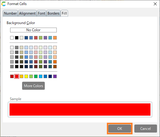
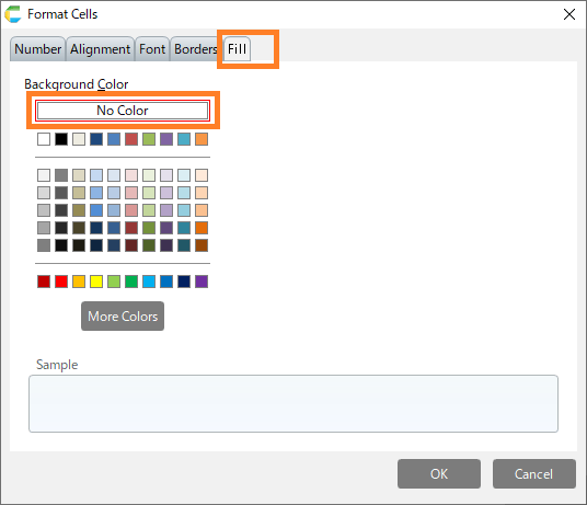
- In the "Fill" tab, edit the "Cells shading color" item as follows
- Cells shading color: red
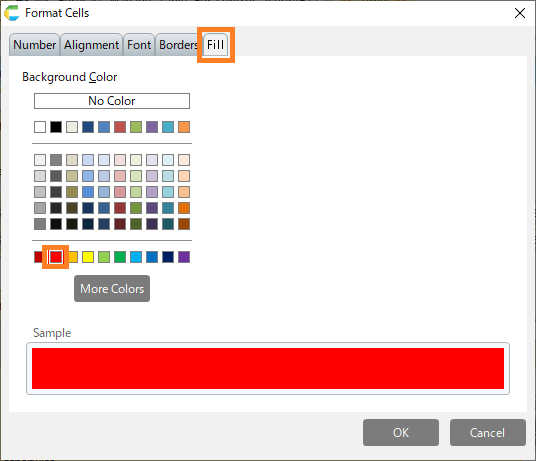
- Click the "OK" button.
Hint
The formatting is now complete.
- Copy the added "Set cell format" action by dragging and dropping it into the "otherwise" part of the "Determine condition" action.
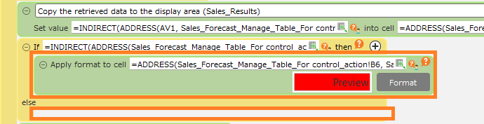
Hint
You can copy an action by dragging and dropping it while holding down Ctrl.
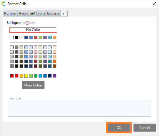
- Click the "Format" button on the copied "Set cell format" action.
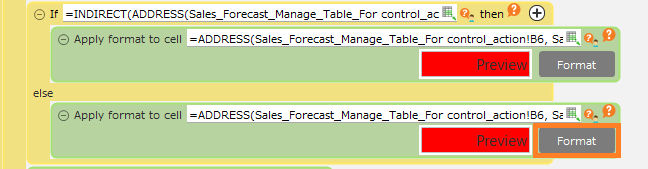
- In the "Fill" tab, edit the "Cells shading color" item as follows
- Cells shading color: No color
- Click the "OK" button.
Hint
The formatting is now complete.
- Click the "OK" button on the action set.
Completed.
See also